eypsurv
This notes demonstrates the basic usage of epysurv
[2]:
import sys
sys.path.append("..")
[3]:
import matplotlib.pyplot as plt
import pandas as pd
from epysurv import data as epidata
[4]:
plt.rc("figure", figsize=(16, 8))
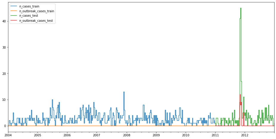
Let’s first get some data and plot it. We use the case counts of Salmonella Newport from Germany between 2004 and 2013. The data is already split into training and test set. We see that there are no outbreaks in the training set, but some around the end of 2011 in the test set.
[5]:
train, test = epidata.salmonella()
train.head()
[5]:
| n_cases | n_outbreak_cases | outbreak | |
|---|---|---|---|
| 2004-01-05 | 0 | 0 | False |
| 2004-01-12 | 0 | 0 | False |
| 2004-01-19 | 2 | 0 | False |
| 2004-01-26 | 2 | 0 | False |
| 2004-02-02 | 1 | 0 | False |
[6]:
fig, ax = plt.subplots()
train.add_suffix("_train").plot(drawstyle="steps-post", ax=ax)
test.add_suffix("_test").plot(drawstyle="steps-post", ax=ax)
[6]:
<matplotlib.axes._subplots.AxesSubplot at 0x7f5509f662e8>
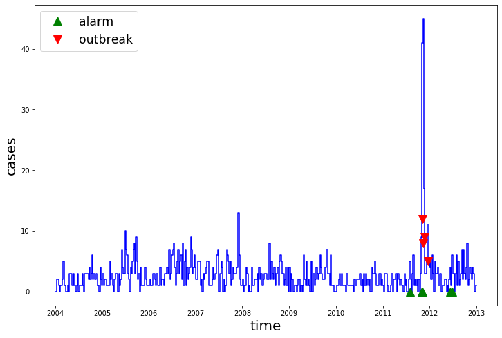
Next we import some classical models: EarsC1 and FarringtonFlexible. The API works really similiar to scikit-learn. Finally, we plot the predictions.
[9]:
from epysurv.models.timepoint import EarsC1, FarringtonFlexible
from epysurv.visualization.model_diagnostics import plot_prediction, plot_confusion_matrix
from sklearn.metrics import confusion_matrix
[10]:
model = EarsC1()
model.fit(train)
pred = model.predict(test)
pred.head()
input
[10]:
| n_cases | n_outbreak_cases | outbreak | alarm | |
|---|---|---|---|---|
| 2011-01-03 | 1 | 0 | False | False |
| 2011-01-10 | 0 | 0 | False | False |
| 2011-01-17 | 3 | 0 | False | False |
| 2011-01-24 | 3 | 0 | False | False |
| 2011-01-31 | 3 | 0 | False | False |
[13]:
pred.query("alarm != 0")
[13]:
| n_cases | n_outbreak_cases | outbreak | alarm | |
|---|---|---|---|---|
| 2011-08-01 | 5 | 0 | False | True |
| 2011-10-31 | 9 | 0 | False | True |
| 2011-11-07 | 41 | 12 | True | True |
| 2012-06-11 | 4 | 0 | False | True |
| 2012-06-25 | 6 | 0 | False | True |
[12]:
plot_prediction(train, test, pred)
[12]:
<matplotlib.axes._subplots.AxesSubplot at 0x7f54c3068ef0>
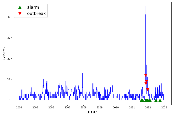
[14]:
model = FarringtonFlexible()
model.fit(train)
pred = model.predict(test)
plot_prediction(train, test, pred)
input
[14]:
<matplotlib.axes._subplots.AxesSubplot at 0x7f54c4255d30>
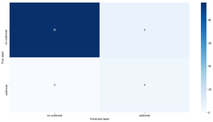
By looking at the confusion matrix, we can see the the FarringtonFlexible successfully detected all outbreak, but also produced some false positives.
[9]:
plot_confusion_matrix(confusion_matrix(test["outbreak"], pred["alarm"]), class_names=["no outbreak", "outbreak"]);
[ ]:
[ ]: